Gradient Descent
We have seen what are the steps followed in Gradient Descent to minimize the loss function. Now let’s get into more detail.
The objective of gradient descent is to find $W, b$ for which $\mathcal{L}(W, b) $ is minimum for given pairs of data $(X, y)$.
Example
Let’s forget about Machine learning for sometime and use gradient descent algorithm for optimization of simple functions.
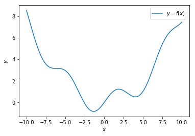
Given a function $y = f(x) = 0.08x^2+sin(x)$, the objective is to find $x$ at which $y = f(x)$ is minimum.
Let’s use Numpy to solve this.
import numpy as np
import matplotlib.pyplot as plt

def f(x):
    return 0.08* x**2 + np.sin(x)

x = np.arange(-10, 10, 0.01)
y = f(x)

plt.plot(x, y, label='$y = f(x)$')
plt.xlabel('$x$')
plt.ylabel('$y$')
plt.legend()
plt.show()
We are going to use gradient descent to find $x$ for which this function is minimum.
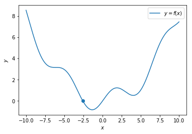
Step - 1
Choose a random point
random_idx = np.random.choice(2000)
random_x = x[random_idx]

plt.plot(x, y, label='$y = f(x)$')
plt.scatter(random_x, f(random_x))
plt.xlabel('$x$')
plt.ylabel('$y$')
plt.legend()
plt.show()
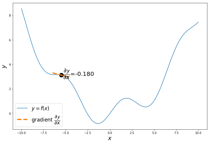
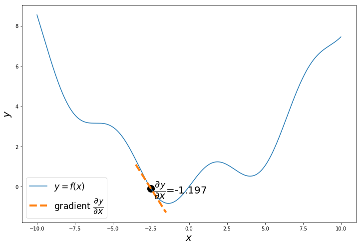
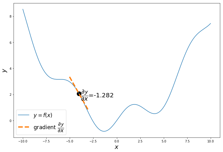
Step - 2
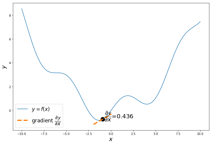
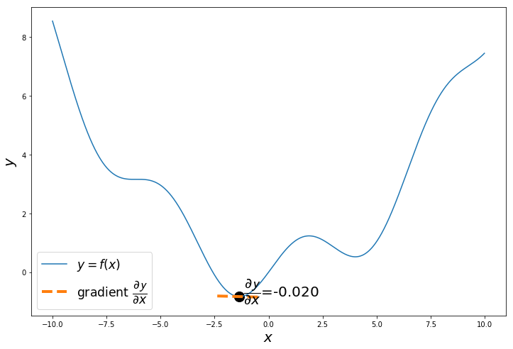
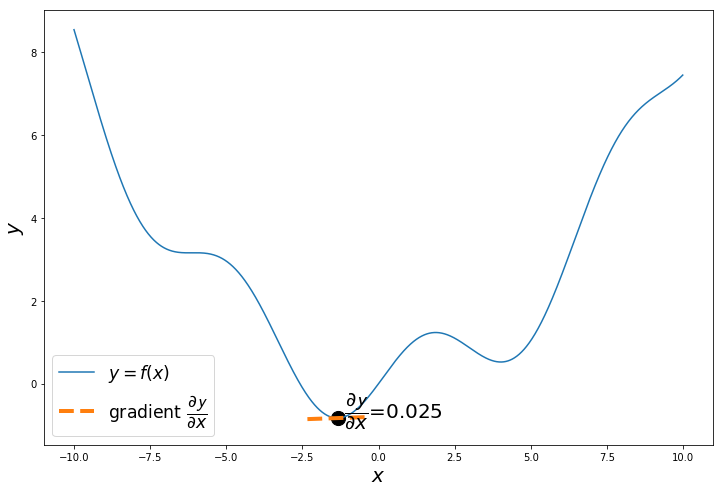
calculate $\dfrac{\partial \mathcal{y}}{\partial x}$.
Why? Let’s visualize it
np.random.seed(60)

random_idx = np.random.choice(2000)
random_x = x[random_idx]

a = random_x
h = 0.01
x_tan = np.arange(a-1, a+1, 0.01)
fprime = (f(a+h)-f(a))/h
tan = f(a)+fprime*(x_tan-a)

plt.figure(figsize=(12,8))
plt.plot(x, y, label='$y = f(x)$')
plt.plot(x_tan, tan, '--', label='gradient $\dfrac{\partial \mathcal{y}}{\partial x}$', linewidth=4.0)
plt.text(a+0.2,f(a+0.2),'$\dfrac{\partial \mathcal{y}}{\partial x}$='+'{:.3f}'.format(fprime), fontsize=20)
plt.scatter(random_x, f(random_x), s=200, color='black')
plt.xlabel('$x$', fontsize=20)
plt.ylabel('$y$', fontsize=20)
plt.legend(fontsize = 'xx-large')
plt.show()
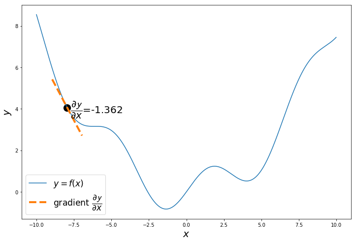
The gradient of $y = f(x) = 0.08x^2+sin(x)$ is $\dfrac{\partial \mathcal{y}}{\partial x} = 0.16x+cos(x)$
The gradient or slope $\dfrac{\partial \mathcal{y}}{\partial x}$ of the curve at the randomly selected point is negative. Which means the function will decrease as x increases and the function will increase as x decreases.
Our objective is to minimize the function, so we calculate $\dfrac{\partial \mathcal{y}}{\partial x}$, to decide in which direction to move, so we reach the minimum.
- if $\dfrac{\partial \mathcal{y}}{\partial x} > 0$, we move towards left of decrease x
- if $\dfrac{\partial \mathcal{y}}{\partial x} < 0$, we move towards right or increase x
- if $\dfrac{\partial \mathcal{y}}{\partial x} = 0$, which means we are already at a point of minimum
But how much to increase x?
Step - 3 Learning rate
We now know, given a point should we increase or decrease x to reach minimum.
How much to increase or decrease x?
We change x with a factor called learning rate $\alpha$. So we update x with $x := x - \alpha \frac{\partial \mathcal{y}}{\partial x}$
- when $\alpha$ is small, x is increased in small steps, so more iterations are required to reach minimum, but this will lead to more accurate steps.
- when $\alpha$ is larger, x will increase in larger steps, so x will reach minimum y in few steps, but there is a risk of x skipping the minimum point, as x is increased in larger value.
When do we stop? We can iterate of any number of iterations, but when x reaches minimum y , then $\dfrac{\partial \mathcal{y}}{\partial x} = 0$
$\therefore x := x - \alpha . 0$, so x will remain the same, even if you iterate more.
Let’s code this.
import numpy as np

def gradient(x):
    return 0.16*x+np.cos(x)
np.random.seed(24) # change the seed to start from different points

x = np.arange(-10, 10, 0.01)
y = f(x)

random_idx = np.random.choice(2000)
x_iter = x[random_idx]

epochs = 100
lr = 0.2

for i in range(epochs):
    dy_dx = gradient(x_iter)
    x_iter = x_iter - lr * dy_dx


    if i%20 == 0:
        a = x_iter
        h = 0.01
        x_tan = np.arange(a-1, a+1, 0.01)
        fprime = (f(a+h)-f(a))/h
        tan = f(a)+fprime*(x_tan-a)

        plt.figure(figsize=(12,8))
        plt.plot(x, y, label='$y = f(x)$')
        plt.plot(x_tan, tan, '--', label='gradient $\dfrac{\partial \mathcal{y}}{\partial x}$', linewidth=4.0)
        plt.text(a+0.2,f(a+0.2),'$\dfrac{\partial \mathcal{y}}{\partial x}$='+'{:.3f}'.format(fprime), fontsize=20)
        plt.scatter(a, f(a), s=200, color='black')
        plt.xlabel('$x$', fontsize=20)
        plt.ylabel('$y$', fontsize=20)
        plt.legend(fontsize = 'xx-large')
        plt.show()


np.random.seed(24) # change the seed to start from different points
x = np.arange(-10, 10, 0.01)
y = f(x)
random_idx = np.random.choice(2000)
x_iter = x[random_idx]
epochs = 100
lr = 0.2
x_list = []
y_list = []
for i in range(epochs):
dy_dx = gradient(x_iter)
x_iter = x_iter - lr * dy_dx
x_list.append(x_iter)
y_list.append(f(x_iter))
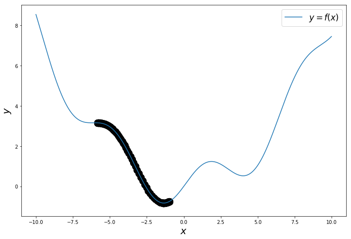
plt.figure(figsize=(12,8))
plt.plot(x, y, label='$y = f(x)$')
for i in range(len(x_list)):
plt.scatter(x_list[i], y_list[i], s=200, color='black')
plt.xlabel('$x$', fontsize=20)
plt.ylabel('$y$', fontsize=20)
plt.legend(fontsize = 'xx-large')
plt.show()
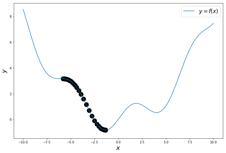
This is the path followed to reach the minimum.
Run the code with
- large lr
- small lr
- more epochs
- less epochs
GD with Momentum
The updation step is changed with
$v = \beta v + (1-\beta) \dfrac{\partial \mathcal{y}}{\partial x}$
$x = x - \alpha v$
This algorithms smoothens the updation process, by averaging the movement in other the direction and forces x to move in the required direction which fastens the process.
Momentum in Numpy
np.random.seed(23) # change the seed to start from different points

x = np.arange(-10, 10, 0.01)
y = f(x)

random_idx = np.random.choice(2000)
x_iter = x[random_idx]

epochs = 100
lr = 0.2
v = 0
b = 0.9

for i in range(epochs):
    dy_dx = gradient(x_iter)
    v = b * v + (1-b) *  dy_dx
    x_iter = x_iter - lr * v


    if i%20 == 0:
        a = x_iter
        h = 0.01
        x_tan = np.arange(a-1, a+1, 0.01)
        fprime = (f(a+h)-f(a))/h
        tan = f(a)+fprime*(x_tan-a)

        plt.figure(figsize=(12,8))
        plt.plot(x, y, label='$y = f(x)$')
        plt.plot(x_tan, tan, '--', label='gradient $\dfrac{\partial \mathcal{y}}{\partial x}$', linewidth=4.0)
        plt.text(a+0.2,f(a+0.2),'$\dfrac{\partial \mathcal{y}}{\partial x}$='+'{:.3f}'.format(fprime), fontsize=20)
        plt.scatter(a, f(a), s=200, color='black')
        plt.xlabel('$x$', fontsize=20)
        plt.ylabel('$y$', fontsize=20)
        plt.legend(fontsize = 'xx-large')
        plt.show()

np.random.seed(24) # change the seed to start from different points

x = np.arange(-10, 10, 0.01)
y = f(x)

random_idx = np.random.choice(2000)
x_iter = x[random_idx]

epochs = 200
lr = 0.1
v = 0
b = 0.9

x_list = []
y_list = []

for i in range(epochs):
    dy_dx = gradient(x_iter)

    v = b * v + (1-b) *  dy_dx
    x_iter = x_iter - lr * v

    x_list.append(x_iter)
    y_list.append(f(x_iter))

plt.figure(figsize=(12,8))
plt.plot(x, y, label='$y = f(x)$')
for i in range(len(x_list)):
    plt.scatter(x_list[i], y_list[i], s=200, color='black')
plt.xlabel('$x$', fontsize=20)
plt.ylabel('$y$', fontsize=20)
plt.legend(fontsize = 'xx-large')
plt.show()
Optimization algorithms with Tensorflow
Check the Tensorflow docs.
So far we have been using ‘Adam’ algorithm for optimization with default parameter values. We will now train models with different optimizers and hyper parameters.
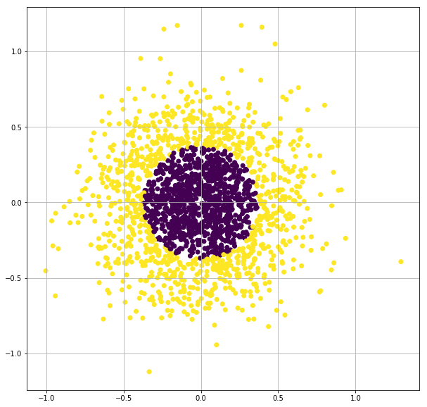
from sklearn.datasets import make_gaussian_quantiles
from sklearn.model_selection import train_test_split
import matplotlib.pyplot as plt

X, y = make_gaussian_quantiles(n_samples=2000, n_features=2, n_classes=2, random_state=3, cov=0.1)

plt.figure(figsize=(10,10))
plt.scatter(X[:,0], X[:,1],c=y)
plt.grid(True)
plt.show()


X_train, X_test, y_train, y_test = train_test_split(X, y, test_size=0.3, shuffle=True)
X_train, X_val, y_train, y_val = train_test_split(X_train, y_train, test_size=0.2, shuffle=True)

print('Train = {}\nTest = {}\nVal = {}'.format(len(X_train), len(X_test), len(X_val)))
Train = 1120
Test = 600
Val = 280
SGD optimizer
Stochastic gradient descent without momentum
import tensorflow as tf
from tensorflow import keras
import numpy as np
import matplotlib.pyplot as plt
tf.keras.backend.clear_session()

# random number initialized to same, for reproducing the same results.
np.random.seed(0)
tf.set_random_seed(0)

model = tf.keras.Sequential([
                             keras.layers.Dense(units=10, input_shape=[2]),
                             keras.layers.Activation('tanh'),
                             keras.layers.Dense(units=10),
                             keras.layers.Activation('tanh'),
                             keras.layers.Dense(units=1),
                             keras.layers.Activation('sigmoid')
                             ])

# we used the default optimizer parameters by using optimizer='adam'
# model.compile(optimizer='adam', loss='binary_crossentropy', metrics=['accuracy'])

# we can also define optimizer with
optimizer = tf.keras.optimizers.SGD(lr=0.01, nesterov=False)
model.compile(optimizer=optimizer, loss='binary_crossentropy', metrics=['accuracy'])
tf_history = model.fit(X_train, y_train, batch_size=100, epochs=50, verbose=True, validation_data=(X_val, y_val))


# contour plot
xx, yy = np.mgrid[-1.5:1.5:.01, -1.5:1.5:.01]
grid = np.c_[xx.ravel(), yy.ravel()]
probs = model.predict(grid)[:,0].reshape(xx.shape)

f, ax = plt.subplots(figsize=(8, 6))
contour = ax.contourf(xx, yy, probs, 25, cmap="RdBu",
                      vmin=0, vmax=1)
ax_c = f.colorbar(contour)
ax_c.set_label("$P(y = 1)$")
ax_c.set_ticks([0, .25, .5, .75, 1])

ax.scatter(X[:,0], X[:, 1], c=y, s=50,
           cmap="RdBu", vmin=-.2, vmax=1.2,
           edgecolor="white", linewidth=1)

plt.show()

# test accuracy
from sklearn.metrics import accuracy_score
y_test_pred = model.predict(X_test)
test_accuracy = accuracy_score((y_test_pred > 0.5), y_test)

print('\nTest Accuracy = ', test_accuracy)
Train on 1120 samples, validate on 280 samples
Epoch 1/50
1120/1120 [==============================] - 0s 96us/sample - loss: 0.7056 - acc: 0.4991 - val_loss: 0.7119 - val_acc: 0.4536
Epoch 2/50
1120/1120 [==============================] - 0s 20us/sample - loss: 0.7048 - acc: 0.5000 - val_loss: 0.7114 - val_acc: 0.4643
.
.
Epoch 49/50
1120/1120 [==============================] - 0s 19us/sample - loss: 0.6910 - acc: 0.6366 - val_loss: 0.6997 - val_acc: 0.5929
Epoch 50/50
1120/1120 [==============================] - 0s 22us/sample - loss: 0.6910 - acc: 0.6348 - val_loss: 0.6991 - val_acc: 0.5714
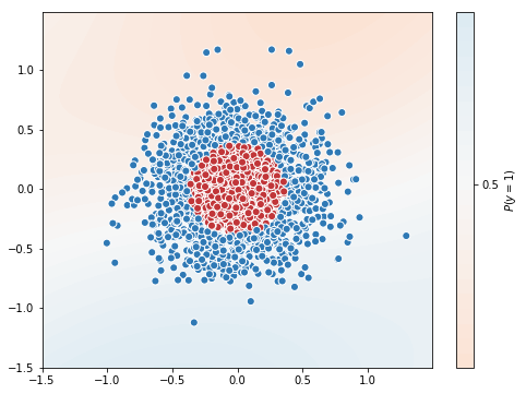
Test Accuracy = 0.6633333333333333
Stochastic gradient descent with momentum
import tensorflow as tf
from tensorflow import keras
import numpy as np
import matplotlib.pyplot as plt
tf.keras.backend.clear_session()

# random number initialized to same, for reproducing the same results.
np.random.seed(0)
tf.set_random_seed(0)

model = tf.keras.Sequential([
                             keras.layers.Dense(units=10, input_shape=[2]),
                             keras.layers.Activation('tanh'),
                             keras.layers.Dense(units=10),
                             keras.layers.Activation('tanh'),
                             keras.layers.Dense(units=1),
                             keras.layers.Activation('sigmoid')
                             ])

# we used the default optimizer parameters by using optimizer='adam'
# model.compile(optimizer='adam', loss='binary_crossentropy', metrics=['accuracy'])

# we can also define optimizer with
optimizer = tf.keras.optimizers.SGD(lr=0.01, momentum=0.9, nesterov=True)
model.compile(optimizer=optimizer, loss='binary_crossentropy', metrics=['accuracy'])
tf_history = model.fit(X_train, y_train, batch_size=100, epochs=50, verbose=True, validation_data=(X_val, y_val))


# contour plot
xx, yy = np.mgrid[-1.5:1.5:.01, -1.5:1.5:.01]
grid = np.c_[xx.ravel(), yy.ravel()]
probs = model.predict(grid)[:,0].reshape(xx.shape)

f, ax = plt.subplots(figsize=(8, 6))
contour = ax.contourf(xx, yy, probs, 25, cmap="RdBu",
                      vmin=0, vmax=1)
ax_c = f.colorbar(contour)
ax_c.set_label("$P(y = 1)$")
ax_c.set_ticks([0, .25, .5, .75, 1])

ax.scatter(X[:,0], X[:, 1], c=y, s=50,
           cmap="RdBu", vmin=-.2, vmax=1.2,
           edgecolor="white", linewidth=1)

plt.show()

# test accuracy
from sklearn.metrics import accuracy_score
y_test_pred = model.predict(X_test)
test_accuracy = accuracy_score((y_test_pred > 0.5), y_test)

print('\nTest Accuracy = ', test_accuracy)
Train on 1120 samples, validate on 280 samples
Epoch 1/50
1120/1120 [==============================] - 0s 104us/sample - loss: 0.7047 - acc: 0.5080 - val_loss: 0.7094 - val_acc: 0.4821
Epoch 2/50
1120/1120 [==============================] - 0s 20us/sample - loss: 0.7002 - acc: 0.5000 - val_loss: 0.7033 - val_acc: 0.4714
.
.
Epoch 49/50
1120/1120 [==============================] - 0s 20us/sample - loss: 0.6351 - acc: 0.7714 - val_loss: 0.6531 - val_acc: 0.7214
Epoch 50/50
1120/1120 [==============================] - 0s 21us/sample - loss: 0.6307 - acc: 0.7750 - val_loss: 0.6463 - val_acc: 0.7393
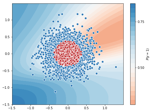
Test Accuracy = 0.7866666666666666
You can note the difference, optimizer with momentum got accuracy of 0.78 in 50 epochs, whereas optimizer without momentum got 0.663 in 50 epochs
Adam optimizer
 Check this paper to know about adam.
import tensorflow as tf
from tensorflow import keras
import numpy as np
import matplotlib.pyplot as plt
tf.keras.backend.clear_session()

# random number initialized to same, for reproducing the same results.
np.random.seed(0)
tf.set_random_seed(0)

model = tf.keras.Sequential([
                             keras.layers.Dense(units=10, input_shape=[2]),
                             keras.layers.Activation('tanh'),
                             keras.layers.Dense(units=10),
                             keras.layers.Activation('tanh'),
                             keras.layers.Dense(units=1),
                             keras.layers.Activation('sigmoid')
                             ])

# we used the default optimizer parameters by using optimizer='adam'
# model.compile(optimizer='adam', loss='binary_crossentropy', metrics=['accuracy'])

# we can also define optimizer with
optimizer = tf.keras.optimizers.Adam(lr=0.01)
model.compile(optimizer=optimizer, loss='binary_crossentropy', metrics=['accuracy'])
tf_history = model.fit(X_train, y_train, batch_size=100, epochs=50, verbose=True, validation_data=(X_val, y_val))


# contour plot
xx, yy = np.mgrid[-1.5:1.5:.01, -1.5:1.5:.01]
grid = np.c_[xx.ravel(), yy.ravel()]
probs = model.predict(grid)[:,0].reshape(xx.shape)

f, ax = plt.subplots(figsize=(8, 6))
contour = ax.contourf(xx, yy, probs, 25, cmap="RdBu",
                      vmin=0, vmax=1)
ax_c = f.colorbar(contour)
ax_c.set_label("$P(y = 1)$")
ax_c.set_ticks([0, .25, .5, .75, 1])

ax.scatter(X[:,0], X[:, 1], c=y, s=50,
           cmap="RdBu", vmin=-.2, vmax=1.2,
           edgecolor="white", linewidth=1)

plt.show()

# test accuracy
from sklearn.metrics import accuracy_score
y_test_pred = model.predict(X_test)
test_accuracy = accuracy_score((y_test_pred > 0.5), y_test)

print('\nTest Accuracy = ', test_accuracy)
Train on 1120 samples, validate on 280 samples
Epoch 1/50
1120/1120 [==============================] - 0s 120us/sample - loss: 0.6971 - acc: 0.5080 - val_loss: 0.6996 - val_acc: 0.6036
Epoch 2/50
1120/1120 [==============================] - 0s 24us/sample - loss: 0.6908 - acc: 0.5545 - val_loss: 0.6979 - val_acc: 0.5357
.
.
Epoch 49/50
1120/1120 [==============================] - 0s 33us/sample - loss: 0.0785 - acc: 0.9804 - val_loss: 0.0694 - val_acc: 0.9821
Epoch 50/50
1120/1120 [==============================] - 0s 25us/sample - loss: 0.0748 - acc: 0.9804 - val_loss: 0.0729 - val_acc: 0.9786
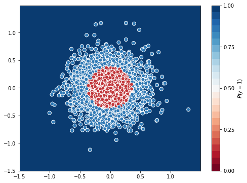
Test Accuracy = 0.9833333333333333
Adam was able to give an accuracy of 0.98 in the same 50 epochs.
So Optimization algorithms affect the learning performance a lot. A good(right) optimization algorithm can improve your performance a lot.
Check out the other optimizers in Tensorflow in the docs.