MNIST Dataset
The MNIST database of handwritten digits, has a training set of 60,000 examples, and a test set of 10,000 examples. It is a subset of a larger set available from NIST. The digits have been size-normalized and centered in a fixed-size image.

Let’s get the dataset using tf.keras.datasets
Download MNIST
import tensorflow as tf

(x_train, y_train), (x_test, y_test) = tf.keras.datasets.mnist.load_data(path='mnist.npz')
Downloading data from https://storage.googleapis.com/tensorflow/tf-keras-datasets/mnist.npz
11493376/11490434 [==============================] - 0s 0us/step
Visualize MNIST
Let’s visualize what is in the dataset
import matplotlib.pyplot as plt

num_imgs = 15
plt.figure(figsize=(num_imgs*2,3))

for i in range(1,num_imgs):
    plt.subplot(1,num_imgs,i).set_title('{}'.format(y_train[i]))
    plt.imshow(x_train[i], cmap='gray')
    plt.axis('off')
plt.show()

Scale the data
import numpy as np

print('Max = {}\nMin = {}'.format(np.max(x_train), np.min(x_train)))
Max = 255
Min = 0
The maximum value in the image if 255 and minimum value is 0. So we need to scale it to a smaller range for faster convergence.
Let’s divide by maximum value of 255, so set it to a range of [0, 1].
x_train = x_train/255
x_test = x_test/255

print('Max = {}\nMin = {}'.format(np.max(x_train), np.min(x_train)))
Max = 1.0
Min = 0.0
One-Hot Encoding
As this is a 10 class multiclass classification, we need to one hot encode the labels.
print(y_train[:5])
[5 0 4 1 9]
num_classes = 10

y_train = tf.keras.utils.to_categorical(y_train, num_classes)
y_test = tf.keras.utils.to_categorical(y_test, num_classes)

print(y_train[:5])
[[0. 0. 0. 0. 0. 1. 0. 0. 0. 0.]
 [1. 0. 0. 0. 0. 0. 0. 0. 0. 0.]
 [0. 0. 0. 0. 1. 0. 0. 0. 0. 0.]
 [0. 1. 0. 0. 0. 0. 0. 0. 0. 0.]
 [0. 0. 0. 0. 0. 0. 0. 0. 0. 1.]]
Flatten
As we are going to use ANNs which takes in vectors and classify/ regress it. But the MNIST images are 2-D matrix, so we cannot directly pass them to ANNs. We need to flatten to the 2-D Matrix to 1-D vectors.
This 3x3 2-D matrix was flattened into a 9 unit vector. So our 28x28 MNIST image will be flattened into a 784 units vector.

x = np.random.randn(3,3)
print(x)
print(x.shape)
print()

flattened_x = x.reshape(-1)
print(flattened_x)
print(flattened_x.shape)
[[-0.09460654  0.70636938 -0.73136131]
 [ 0.9414648   0.89831745 -0.03268361]
 [ 1.27416493 -0.37996    -0.31976928]]
(3, 3)

[-0.09460654  0.70636938 -0.73136131  0.9414648   0.89831745 -0.03268361
  1.27416493 -0.37996    -0.31976928]
(9,)
This can also be done by the model easily with Flatten layer, which we will add to the model.
Model
import tensorflow as tf
from tensorflow import keras

tf.keras.backend.clear_session()

input_shape = (28,28)
nclasses = 10

model = tf.keras.Sequential([
                             tf.keras.layers.Flatten(input_shape=input_shape),
                             tf.keras.layers.Dense(units=50),
                             tf.keras.layers.Activation('tanh'),
                             tf.keras.layers.Dense(units=50),
                             tf.keras.layers.Activation('tanh'),
                             tf.keras.layers.Dense(units=nclasses),
                             tf.keras.layers.Activation('sigmoid')
                             ])
model.summary()
Model: "sequential"
_________________________________________________________________
Layer (type)                 Output Shape              Param #
=================================================================
flatten (Flatten)            (None, 784)               0
_________________________________________________________________
dense (Dense)                (None, 50)                39250
_________________________________________________________________
activation (Activation)      (None, 50)                0
_________________________________________________________________
dense_1 (Dense)              (None, 50)                2550
_________________________________________________________________
activation_1 (Activation)    (None, 50)                0
_________________________________________________________________
dense_2 (Dense)              (None, 10)                510
_________________________________________________________________
activation_2 (Activation)    (None, 10)                0
=================================================================
Total params: 42,310
Trainable params: 42,310
Non-trainable params: 0
_________________________________________________________________
Training the model
optimizer = tf.keras.optimizers.Adam(lr=0.0005)
model.compile(optimizer=optimizer, loss='categorical_crossentropy', metrics=['accuracy'])
tf_history = model.fit(x_train, y_train, batch_size=100, epochs=100, verbose=True, validation_data=(x_test, y_test))
Train on 60000 samples, validate on 10000 samples
Epoch 1/100
60000/60000 [==============================] - 3s 53us/sample - loss: 0.7443 - acc: 0.8594 - val_loss: 0.3127 - val_acc: 0.9262
Epoch 2/100
60000/60000 [==============================] - 3s 52us/sample - loss: 0.2590 - acc: 0.9319 - val_loss: 0.2154 - val_acc: 0.9402
.
.
Epoch 99/100
60000/60000 [==============================] - 3s 51us/sample - loss: 9.9574e-05 - acc: 1.0000 - val_loss: 0.1855 - val_acc: 0.9722
Epoch 100/100
60000/60000 [==============================] - 3s 49us/sample - loss: 9.1121e-05 - acc: 1.0000 - val_loss: 0.1879 - val_acc: 0.9719
plt.figure(figsize=(20,7))

plt.subplot(1,2,1)
plt.plot(tf_history.history['loss'], label='Training Loss')
plt.plot(tf_history.history['val_loss'], label='Validation Loss')
plt.legend()

plt.subplot(1,2,2)
plt.plot(tf_history.history['acc'], label='Training Accuracy')
plt.plot(tf_history.history['val_acc'], label='Validation Accuracy')
plt.legend()
plt.show()
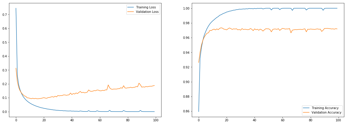
You can observe from this learning curve, as we train more, the training performance improves, but the validation performance goes in reverse direction. This is because the model tries to overfit the training data to improve training data and does not generalize. We have few methods to avoid overfitting. Adding More data always work, but it’s not always possible to get more data, so few regularization techniques may help.
Weight Regularization
$\mathcal{L} = \dfrac{1}{m} \sum_{i=1}^{m}\mathcal{L}(\hat{y}^i, y^i)$
This is the loss which we want to reduce suring gradient descent.
We will add some new terms to the loss function for regularization
$\mathcal{L} = \dfrac{1}{m} \sum_{i=1}^{m}\mathcal{L}(\hat{y}^i, y^i) + \dfrac{\lambda}{2m}\sum_{l=1}^{L}||w^l||^2_2$
where $\lambda$ is called regularization parameter. This is L2 regularization as L2 norm is used.
The objective of any optimization algorithm is to reduce the Loss, now the loss has 2 terms
- MSE or Cross Entropy(can be other loss too)
- Regularization term
To reduce the loss, the optimizer should also reduce $\dfrac{\lambda}{2m}\sum_{l=1}^{L}||w^l||^2_2$ term, which means the weights are also reduced or penalized. How much the weights are penalized depends on $\lambda$, if $\lambda$ is high then the weights are penalized more. Penalizing weights also penalize the activations, which makes a more complex activations to be simpler, so the model does not overfit.
You don’t need to implement it, you can regularize the weights in keras easily with kernel_regularizer.
Regularization in Tensorflow
import tensorflow as tf
from tensorflow import keras

tf.keras.backend.clear_session()

input_shape = (28,28)
nclasses = 10

model = tf.keras.Sequential([
                             tf.keras.layers.Flatten(input_shape=input_shape),
                             tf.keras.layers.Dense(units=50, kernel_regularizer=tf.keras.regularizers.l2(0.0001)),
                             tf.keras.layers.Activation('tanh'),
                             tf.keras.layers.Dense(units=50, kernel_regularizer=tf.keras.regularizers.l2(0.0001)),
                             tf.keras.layers.Activation('tanh'),
                             tf.keras.layers.Dense(units=nclasses),
                             tf.keras.layers.Activation('sigmoid')
                             ])
model.summary()
Model: "sequential"
_________________________________________________________________
Layer (type)                 Output Shape              Param #
=================================================================
flatten (Flatten)            (None, 784)               0
_________________________________________________________________
dense (Dense)                (None, 50)                39250
_________________________________________________________________
activation (Activation)      (None, 50)                0
_________________________________________________________________
dense_1 (Dense)              (None, 50)                2550
_________________________________________________________________
activation_1 (Activation)    (None, 50)                0
_________________________________________________________________
dense_2 (Dense)              (None, 10)                510
_________________________________________________________________
activation_2 (Activation)    (None, 10)                0
=================================================================
Total params: 42,310
Trainable params: 42,310
Non-trainable params: 0
_________________________________________________________________
optimizer = tf.keras.optimizers.Adam(lr=0.0005)
model.compile(optimizer=optimizer, loss='categorical_crossentropy', metrics=['accuracy'])
tf_history_reg = model.fit(x_train, y_train, batch_size=100, epochs=100, verbose=True, validation_data=(x_test, y_test))
Train on 60000 samples, validate on 10000 samples
Epoch 1/100
60000/60000 [==============================] - 3s 55us/sample - loss: 0.7775 - acc: 0.8574 - val_loss: 0.3297 - val_acc: 0.9241
Epoch 2/100
60000/60000 [==============================] - 3s 52us/sample - loss: 0.2782 - acc: 0.9320 - val_loss: 0.2294 - val_acc: 0.9450
.
.
Epoch 99/100
60000/60000 [==============================] - 3s 52us/sample - loss: 0.0249 - acc: 0.9988 - val_loss: 0.1390 - val_acc: 0.9724
Epoch 100/100
60000/60000 [==============================] - 3s 52us/sample - loss: 0.0279 - acc: 0.9977 - val_loss: 0.1359 - val_acc: 0.9741
plt.figure(figsize=(20,7))

plt.subplot(1,2,1)
plt.plot(tf_history.history['loss'], label='Training Loss')
plt.plot(tf_history.history['val_loss'], label='Validation Loss')
plt.plot(tf_history_reg.history['loss'], label='Training Loss with Reg')
plt.plot(tf_history_reg.history['val_loss'], label='Validation Loss with Reg', linestyle='--')
plt.legend()

plt.subplot(1,2,2)
plt.plot(tf_history.history['acc'], label='Training Accuracy')
plt.plot(tf_history.history['val_acc'], label='Validation Accuracy')
plt.plot(tf_history_reg.history['acc'], label='Training Accuracy with Reg')
plt.plot(tf_history_reg.history['val_acc'], label='Validation Accuracy with Reg', linestyle='--')
plt.legend()
plt.show()
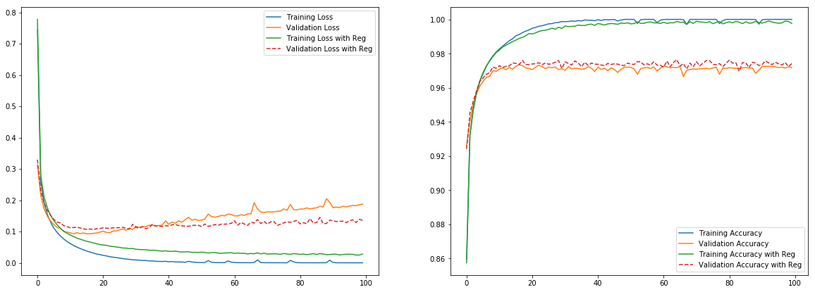
L2 Regularization slightly improved the performance on validation set.
Try changing the l2 regularization $\lambda$ and observe the performance.
Dropouts
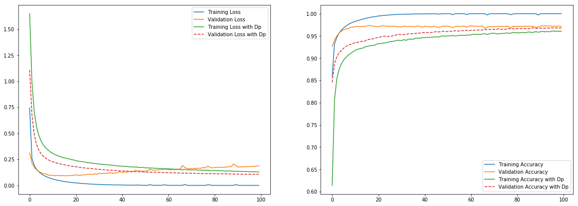
Dropout drops certain nodes in our network during each pass with a defined probability p. So if p=0.5, then each node have a probability of 0.5 to get dropped.
This will make the network simpler during each pass depending on p and now the network cannot rely on any node as it may be dropped, so the network will not give high weights to any node as it may be dropped any time and every node will be utilized equally as all of them have equal probability of being dropped.

Again this can be easily used in keras with tf.keras.layers.Dropout(p).
Dropouts in Tensorflow
import tensorflow as tf
from tensorflow import keras

tf.keras.backend.clear_session()

input_shape = (28,28)
nclasses = 10

model = tf.keras.Sequential([
                             tf.keras.layers.Flatten(input_shape=input_shape),
                             tf.keras.layers.Dense(units=50),
                             tf.keras.layers.Activation('tanh'),
                             tf.keras.layers.Dropout(0.2),
                             tf.keras.layers.Dense(units=50),
                             tf.keras.layers.Activation('tanh'),
                             tf.keras.layers.Dropout(0.2),
                             tf.keras.layers.Dense(units=nclasses),
                             tf.keras.layers.Activation('sigmoid')
                             ])
model.summary()
Model: "sequential"
_________________________________________________________________
Layer (type)                 Output Shape              Param #
=================================================================
flatten (Flatten)            (None, 784)               0
_________________________________________________________________
dense (Dense)                (None, 50)                39250
_________________________________________________________________
activation (Activation)      (None, 50)                0
_________________________________________________________________
dropout (Dropout)            (None, 50)                0
_________________________________________________________________
dense_1 (Dense)              (None, 50)                2550
_________________________________________________________________
activation_1 (Activation)    (None, 50)                0
_________________________________________________________________
dropout_1 (Dropout)          (None, 50)                0
_________________________________________________________________
dense_2 (Dense)              (None, 10)                510
_________________________________________________________________
activation_2 (Activation)    (None, 10)                0
=================================================================
Total params: 42,310
Trainable params: 42,310
Non-trainable params: 0
_________________________________________________________________
optimizer = tf.keras.optimizers.Adam(lr=0.0001)
model.compile(optimizer=optimizer, loss='categorical_crossentropy', metrics=['accuracy'])
tf_history_dp = model.fit(x_train, y_train, batch_size=100, epochs=100, verbose=True, validation_data=(x_test, y_test))
Train on 60000 samples, validate on 10000 samples
Epoch 1/100
60000/60000 [==============================] - 4s 60us/sample - loss: 1.6479 - acc: 0.6138 - val_loss: 1.1078 - val_acc: 0.8455
Epoch 2/100
60000/60000 [==============================] - 3s 53us/sample - loss: 0.9871 - acc: 0.8051 - val_loss: 0.6767 - val_acc: 0.8874
.
.
Epoch 99/100
60000/60000 [==============================] - 3s 54us/sample - loss: 0.1294 - acc: 0.9605 - val_loss: 0.1068 - val_acc: 0.9677
Epoch 100/100
60000/60000 [==============================] - 3s 55us/sample - loss: 0.1294 - acc: 0.9605 - val_loss: 0.1065 - val_acc: 0.9680
plt.figure(figsize=(20,7))

plt.subplot(1,2,1)
plt.plot(tf_history.history['loss'], label='Training Loss')
plt.plot(tf_history.history['val_loss'], label='Validation Loss')
plt.plot(tf_history_dp.history['loss'], label='Training Loss with Dp')
plt.plot(tf_history_dp.history['val_loss'], label='Validation Loss with Dp', linestyle='--')
plt.legend()

plt.subplot(1,2,2)
plt.plot(tf_history.history['acc'], label='Training Accuracy')
plt.plot(tf_history.history['val_acc'], label='Validation Accuracy')
plt.plot(tf_history_dp.history['acc'], label='Training Accuracy with Dp')
plt.plot(tf_history_dp.history['val_acc'], label='Validation Accuracy with Dp', linestyle='--')
plt.legend()
plt.show()