Learning Rate
In Gradient Descent we update the parameters of the model with
$w := w - \alpha \frac{\partial \mathcal{L}}{\partial w}$ and $b := b - \alpha \frac{\partial \mathcal{L}}{\partial b}$.
The learning rate $\alpha$ actually affects the learning process a lot.
- small $\alpha$ is slow, but more accurate, as it does not miss the minimum, but it also get stuck in a local minimum.
- larger $\alpha$ make huge steps, sometimes it may converge faster but it may miss the minima.
Learning rate is an important hyper parameter in training a Model. It is important to understand how to tune the learning rate.
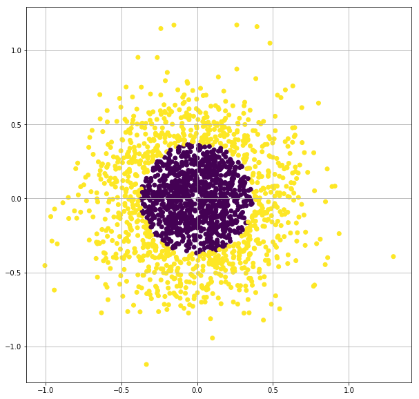
from sklearn.datasets import make_gaussian_quantiles
from sklearn.model_selection import train_test_split
import matplotlib.pyplot as plt

X, y = make_gaussian_quantiles(n_samples=2000, n_features=2, n_classes=2, random_state=3, cov=0.1)

plt.figure(figsize=(10,10))
plt.scatter(X[:,0], X[:,1],c=y)
plt.grid(True)
plt.show()


X_train, X_test, y_train, y_test = train_test_split(X, y, test_size=0.3, shuffle=True)
X_train, X_val, y_train, y_val = train_test_split(X_train, y_train, test_size=0.2, shuffle=True)

print('Train = {}\nTest = {}\nVal = {}'.format(len(X_train), len(X_test), len(X_val)))
Train = 1120
Test = 600
Val = 280
Large Learning rate
We will use adam optimizer with learning rate of 0.5
import tensorflow as tf
from tensorflow import keras
import numpy as np
import matplotlib.pyplot as plt
tf.keras.backend.clear_session()

# random number initialized to same, for reproducing the same results.
np.random.seed(0)
tf.set_random_seed(0)

model = tf.keras.Sequential([
                             keras.layers.Dense(units=10, input_shape=[2]),
                             keras.layers.Activation('tanh'),
                             keras.layers.Dense(units=10),
                             keras.layers.Activation('tanh'),
                             keras.layers.Dense(units=1),
                             keras.layers.Activation('sigmoid')
                             ])

# we used the default optimizer parameters by using optimizer='adam'
# model.compile(optimizer='adam', loss='binary_crossentropy', metrics=['accuracy'])

# we can also define optimizer with
optimizer = tf.keras.optimizers.Adam(lr=0.5)
model.compile(optimizer=optimizer, loss='binary_crossentropy', metrics=['accuracy'])
tf_history = model.fit(X_train, y_train, batch_size=100, epochs=50, verbose=True, validation_data=(X_val, y_val))


# contour plot
xx, yy = np.mgrid[-1.5:1.5:.01, -1.5:1.5:.01]
grid = np.c_[xx.ravel(), yy.ravel()]
probs = model.predict(grid)[:,0].reshape(xx.shape)

f, ax = plt.subplots(figsize=(8, 6))
contour = ax.contourf(xx, yy, probs, 25, cmap="RdBu",
                      vmin=0, vmax=1)
ax_c = f.colorbar(contour)
ax_c.set_label("$P(y = 1)$")
ax_c.set_ticks([0, .25, .5, .75, 1])

ax.scatter(X[:,0], X[:, 1], c=y, s=50,
           cmap="RdBu", vmin=-.2, vmax=1.2,
           edgecolor="white", linewidth=1)

plt.show()

# test accuracy
from sklearn.metrics import accuracy_score
y_test_pred = model.predict(X_test)
test_accuracy = accuracy_score((y_test_pred > 0.5), y_test)

print('\nTest Accuracy = ', test_accuracy)
WARNING: Logging before flag parsing goes to stderr.
W0903 06:12:55.336309 139678620190592 deprecation.py:506] From /usr/local/lib/python3.6/dist-packages/tensorflow/python/ops/init_ops.py:1251: calling VarianceScaling.__init__ (from tensorflow.python.ops.init_ops) with dtype is deprecated and will be removed in a future version.
Instructions for updating:
Call initializer instance with the dtype argument instead of passing it to the constructor
W0903 06:12:55.442114 139678620190592 deprecation.py:323] From /usr/local/lib/python3.6/dist-packages/tensorflow/python/ops/nn_impl.py:180: add_dispatch_support.<locals>.wrapper (from tensorflow.python.ops.array_ops) is deprecated and will be removed in a future version.
Instructions for updating:
Use tf.where in 2.0, which has the same broadcast rule as np.where


Train on 1120 samples, validate on 280 samples
Epoch 1/50
1120/1120 [==============================] - 0s 130us/sample - loss: 0.8366 - acc: 0.4786 - val_loss: 0.7390 - val_acc: 0.4464
Epoch 2/50
1120/1120 [==============================] - 0s 22us/sample - loss: 0.7115 - acc: 0.4902 - val_loss: 0.7462 - val_acc: 0.4464
.
.
Epoch 49/50
1120/1120 [==============================] - 0s 23us/sample - loss: 0.7400 - acc: 0.4920 - val_loss: 0.6896 - val_acc: 0.5536
Epoch 50/50
1120/1120 [==============================] - 0s 22us/sample - loss: 0.7273 - acc: 0.5009 - val_loss: 0.6900 - val_acc: 0.5536
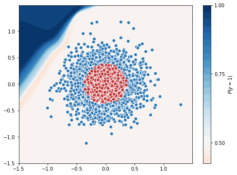
Test Accuracy = 0.49666666666666665
This is one of the worst models you can train, as the learning rate is very high the optimizer skips all the minima and the loss does not really reduces much.
Small Learning rate
We will use adam optimizer with learning rate of 0.00001
import tensorflow as tf
from tensorflow import keras
import numpy as np
import matplotlib.pyplot as plt
tf.keras.backend.clear_session()

# random number initialized to same, for reproducing the same results.
np.random.seed(0)
tf.set_random_seed(0)

model = tf.keras.Sequential([
                             keras.layers.Dense(units=10, input_shape=[2]),
                             keras.layers.Activation('tanh'),
                             keras.layers.Dense(units=10),
                             keras.layers.Activation('tanh'),
                             keras.layers.Dense(units=1),
                             keras.layers.Activation('sigmoid')
                             ])

# we used the default optimizer parameters by using optimizer='adam'
# model.compile(optimizer='adam', loss='binary_crossentropy', metrics=['accuracy'])

# we can also define optimizer with
optimizer = tf.keras.optimizers.Adam(lr=0.00001)
model.compile(optimizer=optimizer, loss='binary_crossentropy', metrics=['accuracy'])
tf_history = model.fit(X_train, y_train, batch_size=100, epochs=50, verbose=True, validation_data=(X_val, y_val))


# contour plot
xx, yy = np.mgrid[-1.5:1.5:.01, -1.5:1.5:.01]
grid = np.c_[xx.ravel(), yy.ravel()]
probs = model.predict(grid)[:,0].reshape(xx.shape)

f, ax = plt.subplots(figsize=(8, 6))
contour = ax.contourf(xx, yy, probs, 25, cmap="RdBu",
                      vmin=0, vmax=1)
ax_c = f.colorbar(contour)
ax_c.set_label("$P(y = 1)$")
ax_c.set_ticks([0, .25, .5, .75, 1])

ax.scatter(X[:,0], X[:, 1], c=y, s=50,
           cmap="RdBu", vmin=-.2, vmax=1.2,
           edgecolor="white", linewidth=1)

plt.show()

# test accuracy
from sklearn.metrics import accuracy_score
y_test_pred = model.predict(X_test)
test_accuracy = accuracy_score((y_test_pred > 0.5), y_test)

print('\nTest Accuracy = ', test_accuracy)
Train on 1120 samples, validate on 280 samples
Epoch 1/50
1120/1120 [==============================] - 0s 108us/sample - loss: 0.7051 - acc: 0.5018 - val_loss: 0.7056 - val_acc: 0.4821
Epoch 2/50
1120/1120 [==============================] - 0s 22us/sample - loss: 0.7050 - acc: 0.5018 - val_loss: 0.7055 - val_acc: 0.4821
.
.
Epoch 49/50
1120/1120 [==============================] - 0s 23us/sample - loss: 0.7027 - acc: 0.5009 - val_loss: 0.7036 - val_acc: 0.4786
Epoch 50/50
1120/1120 [==============================] - 0s 21us/sample - loss: 0.7026 - acc: 0.5009 - val_loss: 0.7035 - val_acc: 0.4786
Test Accuracy = 0.5116666666666667
The loss in this model seems to reduce, but at a very slow rate, so we need to train for more epochs to get a good model.
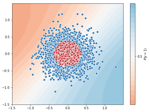
Medium Learning rate
We will use adam optimizer with learning rate of 0.005
import tensorflow as tf
from tensorflow import keras
import numpy as np
import matplotlib.pyplot as plt
tf.keras.backend.clear_session()

# random number initialized to same, for reproducing the same results.
np.random.seed(0)
tf.set_random_seed(0)

model = tf.keras.Sequential([
                             keras.layers.Dense(units=10, input_shape=[2]),
                             keras.layers.Activation('tanh'),
                             keras.layers.Dense(units=10),
                             keras.layers.Activation('tanh'),
                             keras.layers.Dense(units=1),
                             keras.layers.Activation('sigmoid')
                             ])

# we used the default optimizer parameters by using optimizer='adam'
# model.compile(optimizer='adam', loss='binary_crossentropy', metrics=['accuracy'])

# we can also define optimizer with
optimizer = tf.keras.optimizers.Adam(lr=0.005)
model.compile(optimizer=optimizer, loss='binary_crossentropy', metrics=['accuracy'])
tf_history = model.fit(X_train, y_train, batch_size=100, epochs=50, verbose=True, validation_data=(X_val, y_val))


# contour plot
xx, yy = np.mgrid[-1.5:1.5:.01, -1.5:1.5:.01]
grid = np.c_[xx.ravel(), yy.ravel()]
probs = model.predict(grid)[:,0].reshape(xx.shape)

f, ax = plt.subplots(figsize=(8, 6))
contour = ax.contourf(xx, yy, probs, 25, cmap="RdBu",
                      vmin=0, vmax=1)
ax_c = f.colorbar(contour)
ax_c.set_label("$P(y = 1)$")
ax_c.set_ticks([0, .25, .5, .75, 1])

ax.scatter(X[:,0], X[:, 1], c=y, s=50,
           cmap="RdBu", vmin=-.2, vmax=1.2,
           edgecolor="white", linewidth=1)

plt.show()

# test accuracy
from sklearn.metrics import accuracy_score
y_test_pred = model.predict(X_test)
test_accuracy = accuracy_score((y_test_pred > 0.5), y_test)

print('\nTest Accuracy = ', test_accuracy)
Train on 1120 samples, validate on 280 samples
Epoch 1/50
1120/1120 [==============================] - 0s 114us/sample - loss: 0.6968 - acc: 0.5188 - val_loss: 0.6958 - val_acc: 0.3679
Epoch 2/50
1120/1120 [==============================] - 0s 28us/sample - loss: 0.6926 - acc: 0.4098 - val_loss: 0.6941 - val_acc: 0.4643
.
.
Epoch 49/50
1120/1120 [==============================] - 0s 22us/sample - loss: 0.1305 - acc: 0.9652 - val_loss: 0.1324 - val_acc: 0.9607
Epoch 50/50
1120/1120 [==============================] - 0s 22us/sample - loss: 0.1247 - acc: 0.9714 - val_loss: 0.1046 - val_acc: 0.9821
Test Accuracy = 0.96
See how tuning the model from an accuracy of 0.49 to 0.96. Hyper parameter tuning is so critical in getting a good learning model.

Learning Rate Scheduling
We have seen how crucial Learning rate is for training a model. It is also possible that near some minima our optimal learning rate may be big and it doesn’t reach the minima , at that point we may want to reduce the learning rate. This is learning rate scheduling. Instead of using a constant learning rate, we change the learning rate during training to reach the minima.
There are many types of lr scheduling
- step decay
- cosine decay
- reduce on plateau
- cycline decay

LR scheduling can easily be done in Tensorflow
def scheduler(epoch):
  if epoch < 10:
    return 0.001
  else:
    return 0.001 * tf.math.exp(0.1 * (10 - epoch))

callback = tf.keras.callbacks.LearningRateScheduler(scheduler)
model.fit(data, labels, epochs=100, callbacks=[callback],
          validation_data=(val_data, val_labels))
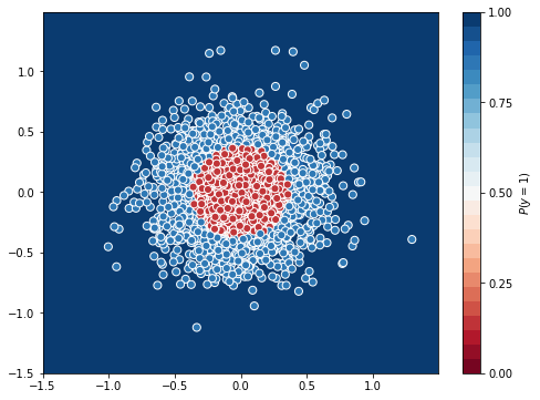
Let’s train a model with ReduceOnPlateau lr scheduling. This checks the loss after every epoch, if the loss is not decreasing for few epochs(say 5) then it reduces the learning by a factor(say 0.1).
ReduceOnPlateau in TensorFlow
import tensorflow as tf
from tensorflow import keras
import numpy as np
import matplotlib.pyplot as plt
tf.keras.backend.clear_session()

# random number initialized to same, for reproducing the same results.
np.random.seed(0)
tf.set_random_seed(0)

model = tf.keras.Sequential([
                             keras.layers.Dense(units=10, input_shape=[2]),
                             keras.layers.Activation('tanh'),
                             keras.layers.Dense(units=10),
                             keras.layers.Activation('tanh'),
                             keras.layers.Dense(units=1),
                             keras.layers.Activation('sigmoid')
                             ])

optimizer = tf.keras.optimizers.Adam(lr=0.05)

from tensorflow.keras.callbacks import ReduceLROnPlateau
reduce_lr = ReduceLROnPlateau(monitor='val_loss', factor=0.5, patience=10, min_lr=0.00001, verbose=True)
model.compile(optimizer=optimizer, loss='binary_crossentropy', metrics=['accuracy'])
tf_history = model.fit(X_train, y_train, batch_size=50, epochs=100, verbose=True, validation_data=(X_val, y_val), callbacks=[reduce_lr])


# contour plot
xx, yy = np.mgrid[-1.5:1.5:.01, -1.5:1.5:.01]
grid = np.c_[xx.ravel(), yy.ravel()]
probs = model.predict(grid)[:,0].reshape(xx.shape)

f, ax = plt.subplots(figsize=(8, 6))
contour = ax.contourf(xx, yy, probs, 25, cmap="RdBu",
                      vmin=0, vmax=1)
ax_c = f.colorbar(contour)
ax_c.set_label("$P(y = 1)$")
ax_c.set_ticks([0, .25, .5, .75, 1])

ax.scatter(X[:,0], X[:, 1], c=y, s=50,
           cmap="RdBu", vmin=-.2, vmax=1.2,
           edgecolor="white", linewidth=1)

plt.show()

# test accuracy
from sklearn.metrics import accuracy_score
y_test_pred = model.predict(X_test)
test_accuracy = accuracy_score((y_test_pred > 0.5), y_test)

print('\nTest Accuracy = ', test_accuracy)
Train on 1120 samples, validate on 280 samples
Epoch 1/100
1120/1120 [==============================] - 0s 156us/sample - loss: 0.6948 - acc: 0.5321 - val_loss: 0.6631 - val_acc: 0.8321
Epoch 2/100
1120/1120 [==============================] - 0s 45us/sample - loss: 0.6391 - acc: 0.6527 - val_loss: 0.6036 - val_acc: 0.7821
.
Epoch 00041: ReduceLROnPlateau reducing learning rate to 0.02500000037252903.
.
Epoch 00078: ReduceLROnPlateau reducing learning rate to 0.012500000186264515.
.
Epoch 00092: ReduceLROnPlateau reducing learning rate to 0.0062500000931322575.
.
Epoch 99/100
1120/1120 [==============================] - 0s 42us/sample - loss: 0.0165 - acc: 0.9955 - val_loss: 0.0202 - val_acc: 0.9857
Epoch 100/100
1120/1120 [==============================] - 0s 43us/sample - loss: 0.0167 - acc: 0.9982 - val_loss: 0.0174 - val_acc: 0.9929

Test Accuracy = 0.9916666666666667
You can see how the learning rates are decreasing when validation loss is not decreasing for 10 steps. Learning rate scheduling will improve the model performance, you will observe it when you train a real world large dataset.